
Introduction
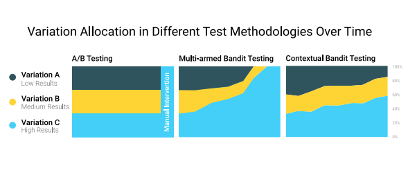
Contextual bandits have become a popular approach to recommender problems, where there are many possible items to offer and there is frequent interaction with the users, e.g. via click/no-click or purchase/no-purchase events. The key idea is that improvement of the recommender policy is achieved in a trial-and-error fashion by taking user features into account. In general, bandit algorithms can be thought of as “online self-improving A/B testing”. A somewhat cartoonish way of comparison of the usual A/B testing, standard multi-armed bandit approach (online improvement not taking individual user features into account) and contextual bandit approach (online improvement taking individual user features into account) could be viewed as follows.
Common applications of contextual bandit algorithms include, among others, news recommendation and website/ad personalization.
In the following we introduce some theory of multi-armed and contextual bandits, and overview their implementations. We also discuss high-level system design of a bandit based recommender system and experiments with actual data.
Multi-armed bandits
The multi-armed bandit problem can be seen as a toy problem for reinforcement learning with one step rollout. Namely we have a game consisting of n rounds and in each round t:
- Player selects one of $K$ actions (think of slot machines and pulling their arms, hence the name).
- Player gets reward of $R_t$. Each action $i\in \{1, 2, …, K\}$ has a fixed, but unknown to the player, reward distribution $P_i$ with the expected reward $\mu_i$.
- Given the history of actions and rewards Player updates their strategy.
The goal of the player is to maximize the reward, which naturally has to be done by exploring new options (and thus learning about other machines' distributions) and exploiting known actions that proved to give high rewards so far. Mathematically the player wishes to minimize the regret
$$R_n := n \mu_* - E[\sum_{t=1}^n R_t],$$
where $\mu_* $ is the expected reward of the best arm (again, a priori this information is obviously unknown) and $E[…]$ is the expected value. Given this data and assuming that the distributions $P_i$ are sufficiently nice (e.g. Gaussian), one can efficiently solve this problem by exploring and exploiting the given actions. Without getting too much into probability theory, one can use concentration inequalities (i.e. how close is the empirical average of rewards for a given action depending on how often I selected it? If did not choose it often enough, I am not sure enough etc.) to construct an algorithm (UCB algorithm) which obtains $R_n$ which grows much more slowly than linearly in $n$, essentially $R_n = O(\sqrt{K n})$. For more details see [1], [2].
(Stochastic) contextual bandits
Multi-armed bandit is a nice introduction to bandit algorithms, however it’s often too simplistic for real world applications. Say we would like to be build a recommender system that should work work with plenty of users and many (possibly varying from round to round) possible actions (actions=arms) to recommend. The multi-armed bandit framework does not cover such situations.
The missing piece is the context (context could be for example user features). For those who know reinforcement learning - one can think of context as “state” (but only the initial state, since we’re still dealing with one step rollouts). Additionally the action set may change from round to round. To make everything clear, here is the core loop for the contextual bandits. We assume that we have a joint distribution $D$ of $(x, R)$, (context, reward) pairs, where R is a sequence of rewards $ \{ R(a) : a \in A \} $, where $A$ is the action set.
$(x_t, R_t) \sim D$ is sampled independently in each round.
- Player gets context $x_t$.
- Player selects $a_t \in A$.
- Player gets reward $R_t(a_t)$. Given the history of actions, rewards and contexts Player updates their strategy.
Note that one usually also assumes that distribution $D = D_t$ changes over time, making the problem non-stationary.
Again, the goal of the player is to maximise the sum of rewards, which can be rewritten mathematically as minimising regret. It is a bit more subtle in this case, since now we are competing not against the best possible policy overall - this is too hard, but against the best policy in a given subclass of policies. Formally, let $\Pi$ be a set of policies that we’re interested in (say neural networks or linear policies) and let $\pi^* \in \Pi$ be the optimal policy, whose expected reward after n rounds is highest. Then, the regret of a sequence of actions $a_t$ is
$$R_n := \sum_{t=1}^n R_t(\pi^* (x_t)) - \sum_{t=1}^b R_t(a_t).$$
Note that such framework does not require us to have a separate bandit algorithm running for each user, since the context can be shared as another input to the algorithm. Although much of theoretical analysis is written in the setting where the action set is finite and fixed, there are practical ways of handling large and changing action sets. Concerning changing sets of actions one usually uses the similar framework, where the player in each gets to see a subset $A_t \subset A$ of actions. Concerning large sets of actions, one usually constructs a feature map $\psi(x_t, a_i) \in \mathbb{R}^d$ for each available action a_i in a given round. $\psi$ can be hand-crafted (e.g. concatenation of $x_t$ and one-hot encoding of each action or interactions of $x_t$ and $a_i$) or learned (e.g. constructed via taking the last hidden layer of neural network pre-trained on some relevant classification problem). In this setting we identify the set of actions with the set of d-dimensional vectors $\{\psi(x_t, a_i) : i \in \{1,2,…,K_t\}\}$ and free ourselves from the number of actions, since now the complexity of the problem is measured in the dimension $d$ instead of $K$.
There are approaches that try to mimic the procedure from the previous section in a $d$-dimensional space (LinUCB algorithm), however they are usually less practical, since they require certain assumptions on the distributions (Gaussian or similar) and inverting high dimensional matrices.
Hence, from now on we will follow [3] and consider the modern approach which uses approximate methods. Essentially all of these methods consists of two steps: explore and learn. We assume that we have access to a model (e.g. linear model or neural net) $f_\theta(x, a)$ parametrized by $\theta$ with inputs $x$ and $a$, which we can update using new data.
In explore phase the algorithm, given its internal estimates of “goodness” of each actions chooses the best possible action modulo exploration. For example, epsilon-greedy chooses the best action with probability $1-\epsilon$ and with probability \epsilon it selects uniformly one of all possible actions.
In the learning phase, the algorithm, after it selects an action and obtains a reward, updates its estimates of expected rewards of actions given the context. This is usually done via feeding a single example consisting of $x$, $a$, $r$ (context, action, reward) to an estimator model doing a single update step (batch size 1). The update step can be something more fancy than the standard SGD, for instance VW (see below) uses AdaGrad. This called a reduction, since we effectively reduce the bandit problem to a cost-sensitive classification problem (we obtain the scores of actions, by querying the estimator for each action). Again, for people knowing RL, the estimator model is essentially the Q-function.
Note that the reduction is a crucial step, since we use partially labeled examples (we obtain feedback only for the selected action) in order to form an estimate of all actions at each time step.
The learn phase is usually common for most algorithms and the main differences come from the exploration phase. Some algorithms considered in [3] are $\epsilon$-greedy, ensemble of policies or approximations to Lin-UCB. $\epsilon$-greedy tends to be a practical choice for initial experiments since it’s straightforward to understand and control its exploration. In particular, initially one can collect more off-policy data for offline evaluation of different, more complex and exploration efficient algorithms to be deployed later on.
Implementations
In the following we use Vowpal Wabbit [14], [15], a machine learning library developed at Microsoft, which contains implementations of state of the art contextual bandit algorithms. It’s implemented in C++, but multiple wrappers (Python, Java, C#) are available.
Concerning other possibilities, very recently researchers from Google published a paper [12] and a blog post [13], where they use Google Cloud AutoML and apply an $\epsilon$-greedy policy with decaying $\epsilon$, and report very good results.
(High-level) system design
Concerning the system design, we will outline the key ideas of the Microsoft Decision Service [4], which is a system for contextual learning, using contextual bandits under the hood.
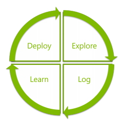
The core loop consists of four steps: exploration, logging, learning and deployment. Exploration and learning correspond to the two steps of the bandit algorithm presented in the previous section, while logging and deployment correspond to logging user interactions and deployment of the updated policy. Note that in a problem where the user rewards can be delayed and computational resources are limited, these two steps are not completely straightforward.
Moreover logging can be later reused for offline experiments. In slightly more details the whole cycle could be viewed as follows.
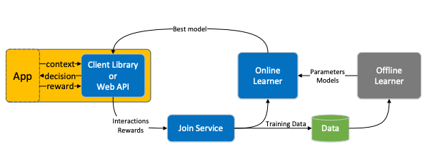
where Join Service is responsive for correctly match the input contexts and actions with the (potentially delayed) rewards. Among others, there are two important problems (and solutions) that come up in a real world scenario.
Delayed rewards. Say a user is offered with an article or a product. In some cases we cannot expect the user to act immediately. The proposed solution is to force uniform delay on all actions, e.g. if there is no click for a given option after 10 minutes, then the default reward of 0 is given. On the other hand, if a click occurs, it’s not processed further until 10 minutes have passed.
Offline evaluation. Say we have exploration data of some policy and want to simulate an experiment with a different policy using only this data. The problem is that the data is only partially labeled (we see feedback only for taken actions) and we want simulate exploration of the new policy, which may be taking different actions than the logged ones. That’s by itself a nontrivial problem and several ides for solving it were proposed [6], [7]. The most effective ones combine importance sampling with smart rejection of certain samples.
Experiments
On one hand contextual bandit algorithms try to reduce the problem to cost-sensitive classification. On the other hand, given a classification dataset one can simulate a contextual bandit problem in the following way, step by step for every example in the dataset:
- We receive $(x, y)$, where x are the features and y is the ground truth label.
- We feed $x$ as the context to the algorithm with the set of actions equal to the set of labels.
- Algorithm proposes one of the labels as the action. If the label is correct, then the reward is $1$, otherwise the reward is $0$.
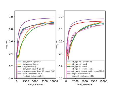
Using such procedure we ran several algorithms on a music genre recommendation dataset, used in the blog post [8]. The algorithms and their hyperparameters were selected according to the extensive analysis of contextual bandit algorithms [3].
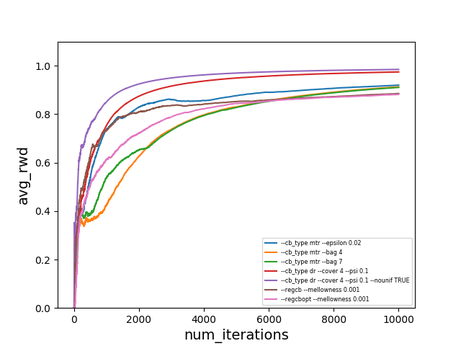
$\text{avg_rwd}(t)$ is the average reward after $t$ iterations ($t$ examples). The dataset does not seem to be particularly hard, but it’s still nice to see that these algorithms work in practice. What’s more interesting is that offline evaluation seems to work as well - of course the estimates are a bit off, but still (surprisingly) close. The results below are on the same dataset with the doubly robust estimator [6]. On the left is the actual performance and on the right is the offline performance of the same algorithms, using the logged data of a different ($\epsilon$-greedy) exploration policy.
Note that there are statistically more sound ways of estimating policies changing over time (which is the case here), called replay [7] (less data efficient) and the doubly robust non-stationary estimator [6] (somewhat more involved).
Real World Use Cases
Contextual bandits were successfully used in many real world situations, for article recommendation at Microsoft [4] and The New York Times [17], for movie recommendation and UI personalization [9], [16] at Netflix. There is also a very relevant use case of contextual bandits for starter pack selection in a mobile game [11].
References
[1] Bandit Algorithms book
[2] Bandit Algorithms slides
[3] A Contextual Bandit Bake-Off paper
[4] Making Contextual Decisions with Low Technical Debt paper
[5] Microsoft Decision Service repository
[6] Doubly Robust Policy Evaluation and Optimization paper
[7] Unbiased Offline Evaluation of Contextual-bandit-based News Article Recommendation Algorithms paper
[8] An Introduction to Contextual Bandits blog post
[9] Machine Learning for Personalization talk
[10] Real World Interactive Learning talk
[11] How We Boosted App Revenue by 10% with Real-time Personalization blog post
[12] AutoML for Contextual Bandits paper
[13] Better bandit building: Advanced personalization the easy way with AutoML Tables blog post
[14] Vowpal Wabbit website
[15] Vowpal Wabbit repository
[16] Artwork personalization blog post
[17] How The New York Times is Experimenting with Recommendation Algorithms